Gaming Virtual Economies

Many video games emphasize economy: rewarding players for providing in-game goods and services for in-game currency. World of Warcraft is one of these games, but it has an interesting component. Players can use a nation’s currency to purchase an in-game token which can then be sold for in-game currency via an auction. Consequentially, that nation’s currency and World of Warcraft gold have an exchange rate at any given moment.
I used this fact to backtest a trading algorithm between national currencies and World of Warcraft gold. The algorithm used an ARIMA prediction model to inform decisions by a currency carry trade strategy. A bisection algorithm was used to optimize volume for each trade.
Backtest
Data
Data came from WoW Token Prices and extended back to April of 2015. Data was available for China (Yuan), Europe (Euro), South Korea (won), Taiwan (New Taiwan Dollar), and the United States (US Dollar). The rates are in 20 minute increments (3 moments per hour, 72 moments per day). The rates are X gold per token. Tokens can cost $15, £20, etc.

Model Design
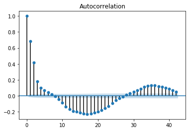
The ARIMA model was fitted using US data from December of 2015 to July of 2016. Per the augmented Dickey-Fuller test, the time series was stationary after one round of differencing, however seasonality was present. Unfortunately, the seasonality was not included in the model because of an issue optimizing those parameters and employing them in the code. Nevertheless, an ARIMA(5,1,5) model was constructed. It was assumed that the autocorrelation after 5 lags was more indicative of seasonality than anything else.


Pricing Functions
To better simulate supply and demand, pricing functions were designed. These were designed such that bang-per-buck decreased with each additional unit.
For gold purchases, each token yields less gold because
the increase in token supply reduces price
reducing token price increases the number of potential buyers.
For gold sales, each token costs more gold
the decrease in token supply increases price
increasing token price increases the number of potential sellers
While some the compound and decay functions are arbitrary, they still limit the amount the algorithm can profit during a trade and emulate microeconomic effects (which was the purpose).
Gold-purchase rate (decay)
Gold-sale rate (compound)
Expected Profit
Expected Profit First Derivative
In order to maximize gains during each trade, a bisection algorithm was employed to solve for the volume (number of tokens) that maximizes profit.
Evaluation Logic
The evaluation was kept simple since bisection is time intensive. Currency carry is a surprisingly intuitive method. If I have 1 USD and I’m looking at the Euros per USD exchange rate, an increase in the rate (Euro inflation, USD deflation, or both) gets me more Euros. A decrease in the rate (Euro deflation, USD inflation, or both) gets me fewer Euros. However, if I buy Euros (sell USD) when the rate is high, then sell Euros (buy USD) when the rate is low, I will have more USD than I started with.
Return to our 1 USD. For this example
The current exchange rate is 1 Euro per USD (1 USD per Euro)
The next exchange rate is 0.5 Euros per USD (2 USD per Euro)
If I buy a Euro now, in a moment, it will be worth 2 USD because I get 1 USD for every 0.5 Euros.
This algorithm compelled all gold purchases to be followed by a gold sale. This prevented any trend in World of Warcraft gold’s value from radically affecting the net worth. This also meant that the ARIMA model only had to predict one step ahead, keeping computations simple and improving speed. However, establishing one currency as the default has its risks; this will be attenuated to in a future version.
Parameters
A few parameters are assumed.
What currency?
Euros
How much money do we begin with?
1000 Euros, 200,00 WoW Gold
How much does a token cost in that currency?
20 Euros
What will the compound rate be for the pricing functions?
0.00001
Results
Financials
The algorithm evaluated over 119,000 moments from April of 2015 to June of 2020. Its performance was commendable. Starting with a net worth of £1107, the algorithm increased its value to £47.3k. With the exception of a few crashes, its performance was consistent. Had the algorithm not been run, the net worth would have depreciated to £1024.

Given the above compounding interest formula, this algorithm's growth is tantamount to
1.12 annual r/n
112% annual interest
0.46 semiannual r/n
46% semiannual interest
0.06 monthly r/n
6% monthly interest
0.002 daily r/n
0.2% daily interest
over the same period of time.
Model & Strategy
An experiments was run to determine the effectiveness of the algorithm’s design.
Experiment 1
The ARIMA model returns a price difference since it is on the order of (5,1,5). We want to test whether the ARIMA’s predicted price difference is a more accurate predictor than the prior price difference.
Hypothesis: ARIMA predictions will be positively related to the true price difference at an alpha of 0.001.
Method:
OLS regression between moment t's predicted price difference and moment t's true price difference.
OLS regression between moment t-1’s price difference and moment t’s true price difference.
Results:
Using the prior value (R-Squared 0.374) would have been more effective than an ARIMA(5,1,5) model’s prediction (R-Squared 0.347).


Performance Time
An important component of any trading algorithm is speed, especially if other algorithms are in the market. While this doesn’t apply to World of Warcraft, it is still a good habit to design as if. Most algorithms are designed in computationally fast languages such as C and C++. This grants them a leg up to design slightly more sophisticated logic and evaluation procedures. One of goals was to design a Python algorithm that is lean and simple.
There are three possible scenarios: buy, sell, or hold. As mentioned in Evaluation Logic, a buy is always followed by a sell. Because sales are reactionary, we expect them to be quicker.

The algorithm’s brevity was impressive for Python. Even during purchase evaluations (when we run the sluggish bisection algorithm), the algorithm was completing most trades around or below 100 microseconds. While this ignores important variables such as network speed, database requests, realtime API calls, etc. Yet it is an auspicious start for an algorithm coded in a language that is notorious for sloth-like execution speeds.
TL;DR
An ARIMA(5,1,5) model was run to predict currency appreciation and depreciation
The currency carry strategy is based upon exploiting momentary appreciation and depreciation.
Net worth went from £1107 to £47.3. If the algorithm was not run, net worth would have depreciated to £1024.
The backtest emulated economic principles to model changes in price according to changes in volume.
The ARIMA model was ineffective. Another modeling strategy will be looked into for future versions.
The algorithm was fast: completing over 99% of decisions within 175 microseconds.